And how naive to have imagined that the series ended at this point, in only three dimensions!
− 2001, A Space Odyssey, by Arthur C. Clarke
The German philosopher-scientist Gottfried Leibniz dreamed of a universal language and a method of calculation to go with it, so that, if disputes arose on any subject, a disputant could exclaim “Calculemus!” (“Let us calculate!”) and the method would yield the answer.
It was an audacious dream and Leibniz knew it, but, hoping to bring one small corner of his dream-language to life, he attempted to invent a “geometry of situation” that would blend algebra and geometry. He adopted ♉︎ (the zodiacal symbol for taurus) to signify the relation of congruence, and he tried to reduce all the traditional notions of geometry to properties of ♉︎.1 Leibniz aimed to devise a kind of “Solid Geometry 2.0” that would allow him and others to reason about geometric situations by first translating the situations into statements involving ♉︎ and then making algebra-style deductions from those statements using suitable axioms.
Leibniz wrote to his friend the Dutch mathematician Christian Huygens in 1679 that he envisioned a language that would describe not just geometry but the actions of machines. “I believe that by this method one could treat mechanics almost like geometry, and one could even test the qualities of materials.” Leibniz failed to convince Huygens and others to help him develop his ideas, but with hindsight we can see glimmerings of the idea of vectors in what he wrote. If only he’d based his system on translational congruence – the relation that holds when one figure can be obtained from another using only sliding, not rotation – he would’ve gotten closer to the modern concept of vectors and everything that the concept led to, including (most recently) chatbots.
At roughly the same time, Leibniz’s English rival Isaac Newton was establishing the principles of Newtonian physics in his great work Principia Mathematica, using classical two- and three-dimensional geometry as a stage upon which new actors named Motion and Force took their places and spoke their lines – portentous lines such as “A body acted on by two forces acting jointly describes the diagonal of a parallelogram in the same time in which it would describe the sides if the forces were acting separately.” Newton saw that the analysis of force requires one to ask both “How strong is the force?” and “In what direction is the force pushing?”, and in that respect, he anticipated the concept of vectors, which are mathematical quantities with both magnitude and direction.
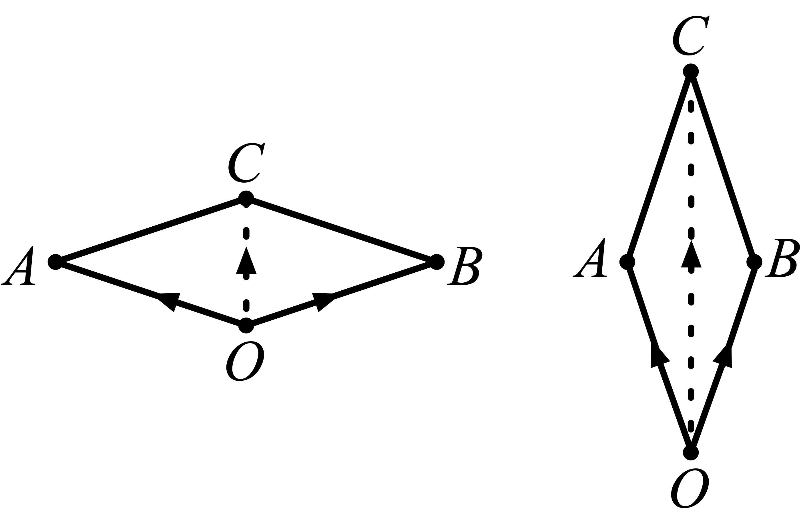
As an example of the way forces combine, imagine two people walking on either side of a canal, holding ropes tethered to a boat. For simplicity, imagine that both ropes are attached at the same point at the prow of the boat. If the walkers walk abreast with one another on opposite sides of the canal and pull with equal force, then the boat will travel straight along the canal, but only some of the muscular effort of the walkers is propelling the boat forward; the rest gets canceled out in a kind of tug-of-war as one walker pulls the boat to the left while the other pulls the boat to the right. The parallelogram law makes this partial cancellation quantitative in a pictorial way. To determine the effective force on the boat, draw parallelogram OABC, where O is the common point of attachment of the ropes at the prow, A and B are the positions of the walkers, and C is the fourth point of the parallelogram. The effective force acting on the boat is proportional to the length of segment OC, so if the two walkers walk only a short way ahead of the boat (as in the left half of the figure), then most of their force is wasted laterally, while if the walkers are far ahead of the boat (as in the right half of the figure), then very little force is wasted. In the latter case, the length of segment OC is almost equal to the sum of the lengths of segments OA and OB, so the force pulling the boat forward is almost as great as if two walkers were miraculously walking on water directly ahead of the boat.
The mathematician Salomon Bochner later wrote: “The Euclidean Space that underlies the Principia is mathematically not quite the same as the Euclidean Space that underlies Greek mathematics (and physics) from Thales to Apollonius. … The Euclidean Space of the Principia continued to be all this, but it was also something new in addition.”
SOMETHING NEW IN ADDITION
A century after Leibniz and Newton, vectors in the strictly mathematical sense were invented in all but name by the Danish-Norwegian mathematician and cartographer Caspar Wessel. Wessel described a way to add straight lines (modern pedants like myself call them line segments) such as AB and CD below.
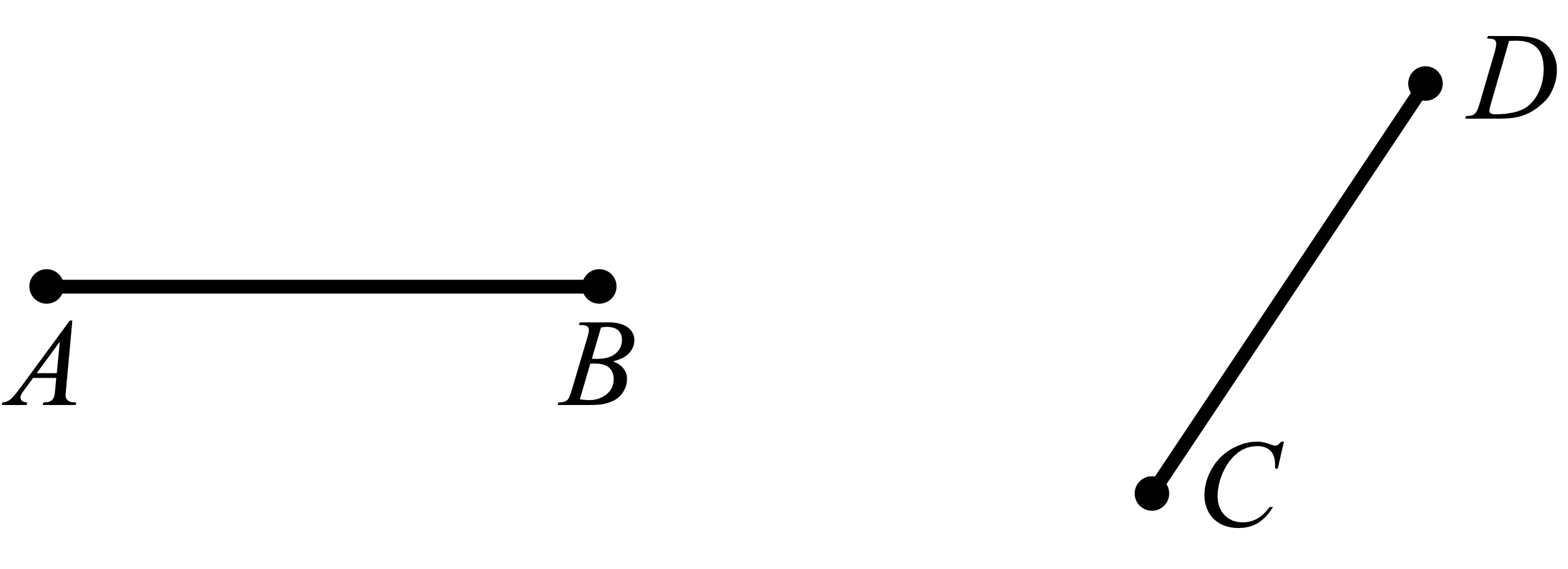
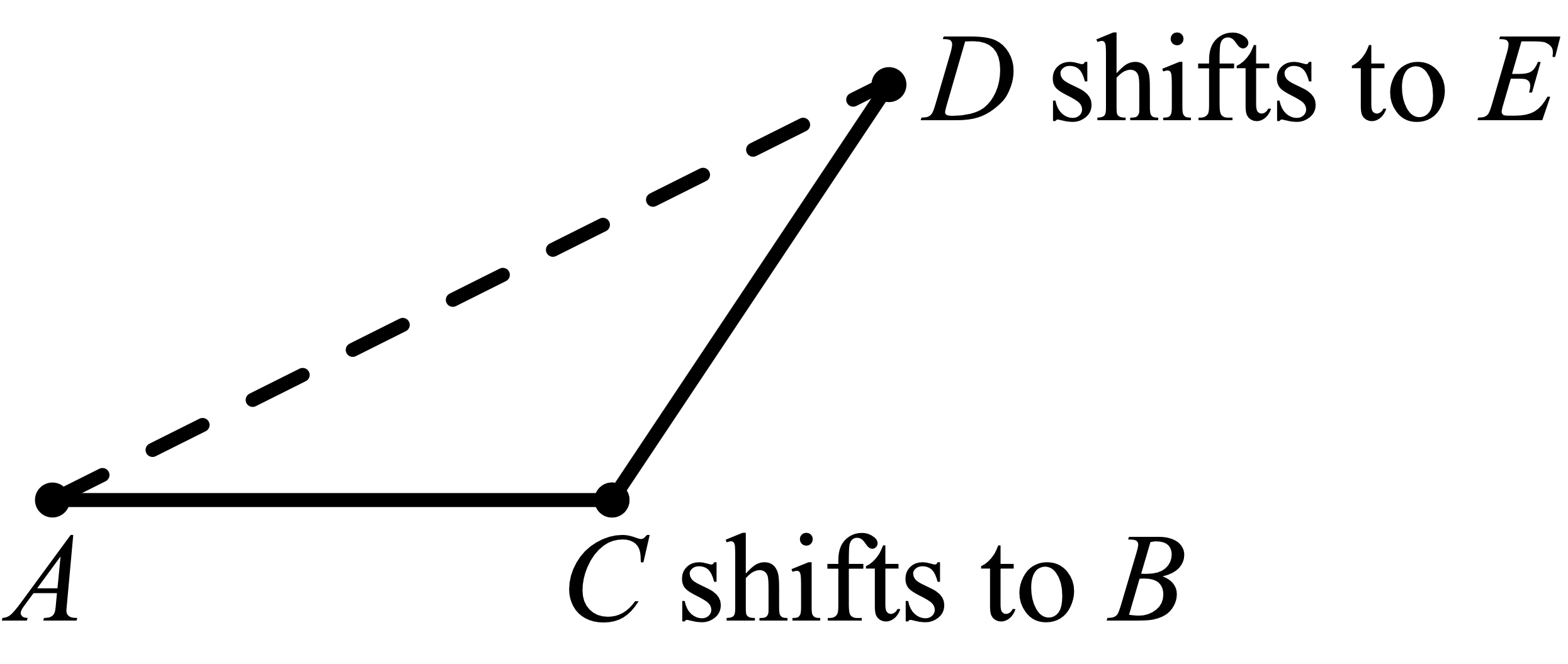
“Two straight lines are added if we unite them in such a way that the second line begins where the first one ends, and then pass a straight line from the first to the last point of the united lines. This line is the sum of the united lines.” Pictorially, we move line segment CD upward and to the left (sliding, not rotating) until C coincides with B, and D as a consequence coincides with some point I’ll call E; then line segment AE is declared to be the sum of line segments AB and CD, as shown below. Note that this is a purely geometric construction, devoid of ideas about velocity, force, etc. though reminiscent of them.
Wessel thinks of A as the “first” point of AB and B as the “last” point and they play different roles in the construction, so in Wessel’s definition AB and BA are not the same; in modern terms, we’d say that Wessel was implicitly working with directed line segments. It’s customary nowadays to adorn an directed line segment with an arrow pointing from where the directed line segment starts to where it ends.
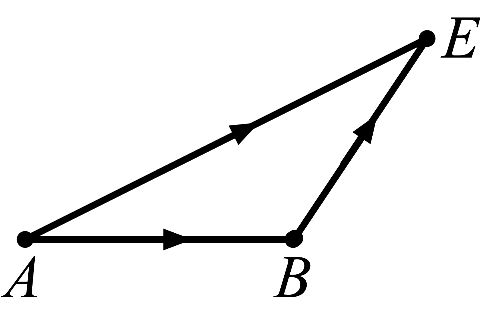
I’ll write A→B to mean “the directed line segment that starts at A and ends at B”. We get an especially nice picture if the second directed line segment already starts where the first directed line segment ends: A→B plus B→C is just A→C.
We also get a nice picture when the starting points of the two directed line segments are the same. To add A→B and A→C, find the point D that completes a parallelogram with points A, B, and C; then the sum of A→B and A→C is A→D, as in the canal boat picture from before.
The arrow picture fails to do justice to an important special case, namely, A→A, a directed line segment that ends where it starts, corresponding to a motion that goes nowhere. In Wessel’s theory, this is the additive identity element: adding it to any directed line segment just gives you that directed line segment back again. Likewise, the directed line segment B→A is the additive inverse of the directed line segment A→B; if you add them in either order, you get the identity element.
Things can get confusing when we work with Cartesian coordinates, since both points and vectors get represented by ordered pairs. The displacement from the point with coordinates (x, y) to the point with coordinates (x′, y′) is a displacement x′−x units to the right and y′−y units upward (with the usual understanding that a negative displacement to the right means a positive displacement to the left and a negative displacement upward means a positive displacement downward); many people (though not all) write this displacement vector as [x′ − x, y′ − y]. In terms of bracketed pairs, Wessel’s addition rule amounts to [a, b] + [c, d] = [a+c, b+d]; that is, if you compound the a-units-over-and-b-units-up displacement and the c-units-over-and-d-units-up displacement, the result is an (a+c)-units-over-and-(b+d)-units-up displacement. Also, notice that [0, 0] is the stay-where-you-are displacement, while [−a, −b] (also written as −[a, b]) is the reversal of [a, b].
Alas, Wessel’s 1797 breakthrough was forgotten until long after its moment to shine had passed.2
VIVE LA DIFFÉRENCE
Another precursor to vectorial theory was the barycentric calculus of August Ferdinand Möbius.3 In 1827, thirty years before he discovered the twisted surface he is famous for nowadays, Möbius came up with a new twist on Archimedes’ method of proving geometrical theorems by way of the branch of physics called statics. Statics is the study of equilibrium, such as the equilibrium of a beam that is perfectly balanced between opposing downward forces on either side of the fulcrum, and Archimedes had made brilliant use of the concept of center-of-gravity to compute the area of a region bounded by an arc of a parabola, among other things.
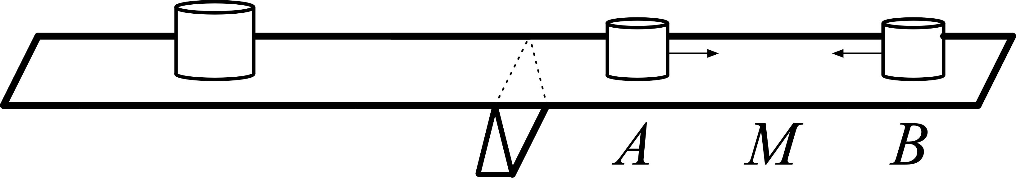
In the barycentric calculus, we can add points, or rather, point-masses, so that for instance 1 unit of mass at some point plus 1 unit of mass at some other point is “equal” to 2 units of mass at the midpoint. To see the physical intuition behind this definition (at least in the case where points A and B and their midpoint M lie on a horizontal line), picture a balance beam supporting 1 unit of mass at A and 1 unit of mass at B, as shown in the picture below. Suppose there’s a fulcrum out to the left and a weight even farther out to the left precisely balancing the combined weights at A and B. Now suppose we slide the weight at A to the right and at the same time slide the weight at B the same distance to the left; the beam will continue to balance because the center of gravity of the two weights is unaffected. When the two masses meet, we will have 2 units of mass at M and the beam will still balance; so 1 unit of mass at A plus 1 unit of mass at B is tantamount to 2 units of mass at the midpoint M. Following Möbius, we write 1A + 1B = 2M. In this particular example A, B, and M lie on a horizontal line, but in Möbius’ actual definition the horizontal line plays no special role.
Möbius’ work languished partly because his methods weren’t relevant to the research priorities of his contemporaries and hence were not deemed useful. Möbius was born a couple of millennia too late (Archimedes would have loved his work) or a couple of centuries too early (high school mathletes exploit the barycentric calculus, re-branded as “mass point geometry”, as a secret weapon4 for solving tricky geometry problems).
The other reason the barycentric calculus didn’t catch on is that even the great mathematicians who learned about it found parts of it confusing. The problem was negative masses. Möbius didn’t just add points; he subtracted them too, even though he had trouble explaining to others what this meant. Consider triangle ABC with midpoints marked along two of the sides (with D halfway between A and B and with E halfway between A and C), as shown below:
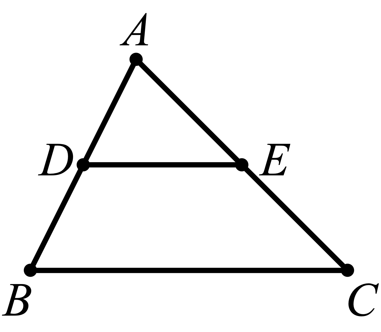
In this picture we have 1A + 1B = 2D and 1A + 1C = 2E, so subtracting the second equation from the first (and canceling the two 1A terms) we get 1B − 1C = 2D − 2E, or 1(B − C) = 2(D − E), which Möbius interpreted to mean that segment BC was parallel to segment DE and twice as long. That’s a nice proof of a true fact, but where are the centers of mass of 1B − 1C and 2D − 2E? Möbius said they were “at infinity”, so you can see why his contemporaries balked.5
SIGNS OF THE TIMES
Yet another prophet of the modern concept of vectors was the German mathematician Hermann Grassmann. His father was the less-well-known mathematician Justus Günther Grassmann, who in an 1824 treatise had written “A rectangle is the geometrical product of its base and height and this product behaves in the same way as the arithmetic product.” The elder Grassmann was not speaking of the lengths of the sides, which are just numbers that one can multiply in the ordinary way; rather, he was speaking of the sides as things in themselves, capable of being multiplied in a geometric manner analogous to, but different from, numerical multiplication of the side-lengths.
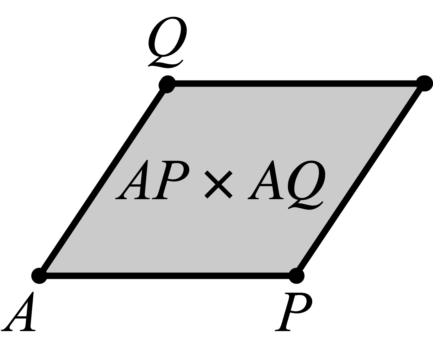
The younger Grassmann extended his father’s idea, saying that all parallelograms, not just rectangles, could be viewed as the product of two directed magnitudes. With this bold step he founded the subject of geometric algebra. But before I say more about that, let me streamline the terminology I’m using, since “directed magnitude” is just as big a mouthful as “directed line segment”. Half a century after Grassmann, authors William Clifford and Karl Pearson, describing Clifford’s version of Grassmann’s work for the lay reader in their book Common Sense of the Exact Sciences6, chose to refer to “directed magnitudes” as just “steps”, and I choose to follow them in this; “step” is a less intimidating word than “vector”! So I say (quoting Clifford and Pearson’s book) that the geometric product of AP and AQ “bids us move the step AQ parallel to itself so that its end A traverses the step AP; the area traced out by AQ during this motion is the value of the product” – although, as we’ll see, the concept of area needed a couple of adjustments before it could fully suit Grassmann’s purposes.
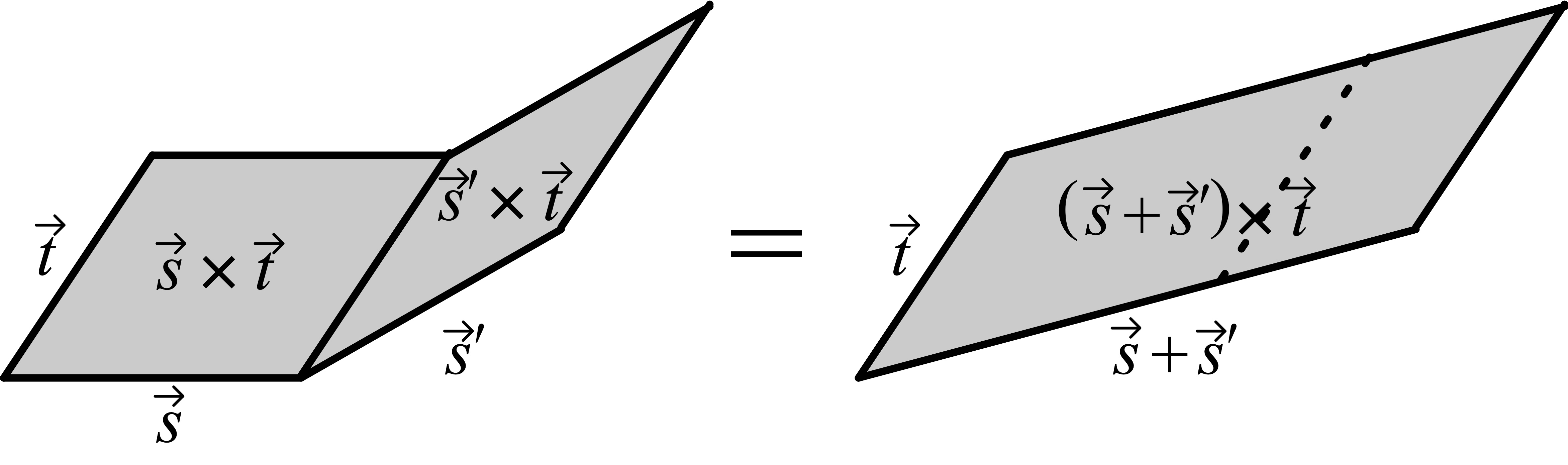
Grassmann reinvented Wessel’s kind of geometric addition (wherein the step from A to B plus the step from B to C equals the step from A to C) and noticed that geometric multiplication was distributive over geometric addition: if s, s‘, and t are steps, (s+s‘) × t equals s × t plus s‘ × t , and likewise s × (t+t‘) equals s × t plus s × t‘. Grassmann took this as an encouraging sign.
But he also realized that the internal logic of his theory required that, far from being commutative, his kind of multiplication had to be anticommutative: changing the order of the two factors caused the geometric product to change sign! That is, the geometric product t × s must be equal to the negative of the geometric product s × t. Grassmann wrote: “I was initially perplexed by the strange result that though the other laws of ordinary multiplication, including the relation of multiplication to addition, were preserved in this new type of multiplication, yet one could only exchange factors if one simultaneously changed the sign, i.e., changed plus to minus and minus to plus.”
To un-perplex ourselves, we can think of this sign-change in connection with the notion of signed area. Clifford and Pearson wrote: “The sign of an area depends upon the way it is gone round; an area gone round counter-clockwise is positive, gone round clockwise is negative.”7

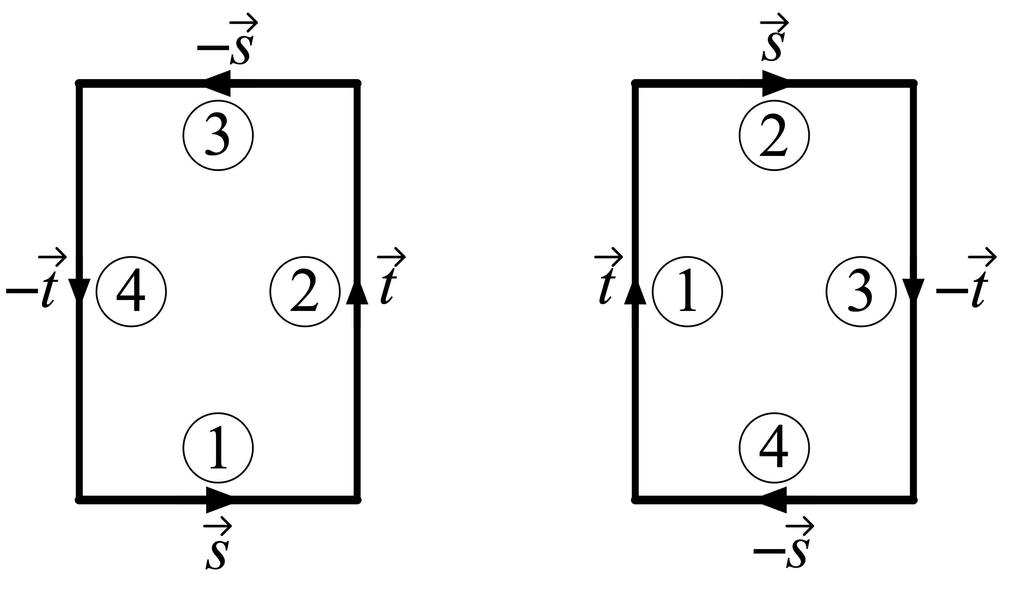
Clifford and Pearson continued: “Although 2 × 2 = 0 and 2 × 3 = −3 × 2 may be sheer nonsense when 2 and 3 are treated as mere numbers, it yet becomes downright common sense when 2 and 3 are treated as directed steps in a plane.” That is: If we replace 2 and 3 by two steps in different directions (call them s and t), and we adopt the convention that the geometric product of the steps s and t corresponds to the parallelogram traced out bytaking the step s, the step t, the step −s, and the step −t in that order, then the s × t parallelogram and the t × s parallelogram have opposite areas (one negative, one positive) because one is traversed clockwise while the other is traversed counterclockwise.
Grassmann’s geometric product (nowadays called the wedge product) isn’t limited to the plane. For instance, in three dimensions the geometric product of two steps is an oriented parallelogram. Technically this product isn’t itself a step because it’s two-dimensional8, but we can represent this parallelogram by a step whose magnitude is proportional to the area of the parallelogram and whose direction is perpendicular to the parallelogram. If we do this, then the product of the step [a, b, c] and the step [a′, b′, c′] turns out to be the step [bc′ − b′c, ca′ − ac′, ab′ − a′b]. This will matter in a little bit.
CHANGING TIMES
Grassmann also defined another way to multiply steps, which he called the linear product. The linear product of the step [a, b, c] and the step [a′, b′, c′] is the number aa′+bb′+cc′. Like his geometric product, Grassmann’s linear product is distributive over addition: if we write the linear product of s and t as s · t (as I’ll do even though Grassmann didn’t), we have (s+s‘) · t = s · t + s‘ · t and s · (t+t‘) = s · t + s · t‘.
The defining rule for linear products is that s · t equals the length of s times the length of t times the cosine of the angle between them. But if you’re rusty on trig, here’s how to think about this:
If s and t point in the exact same direction (that is, if the angle between them is 0 degrees), then the linear product of s and t is just the numerical product of the lengths of those two steps.
If s and t point in opposite directions (that is, if the angle between them is 180 degrees), then the linear product of s and t is the negative of the numerical product of the lengths of those two steps.
For intermediate angles, the linear product of s and t lies between these two extremes, and in particular, if s and t point in perpendicular directions (that is, if the angle between them is 90 degrees), then the linear product of s and t is 0. In this case, we also say that the steps are orthogonal (as heard in such utterances as “Someone who likes continued fractions is neither more likely nor less likely to enjoy eating pickled okra than the average person; the two traits are orthogonal”).
In the case where s = t (and the angle is therefore 0, whose cosine is 1), we see that s · s (the linear product of s with itself) is the squared length of s. This special case is important! It tells us that if we have the linear product, then we have a way of defining length thrown in for free.
With this set-up taken as our foundation, we can derive the Pythagorean Theorem as a consequence.9 Similar reasoning lets us prove in algebraic fashion more complicated facts from geometry, such as the fact that the sum of the squared lengths of the diagonals of a parallelogram equals the sum of the squared lengths of the four sides.10
Grassmann’s system, presented in an 1844 work entitled Linear Extension Theory, a New Branch of Mathematics, isn’t limited to 2- and 3-dimensional geometry; the system encompasses spaces of higher dimension as well. In fact, Grassmann’s formulas give a foundation on which the theory of higher-dimensional Euclidean spaces can be built.11 Unfortunately Grassmann’s ideas, like those of Wessel and Möbius before him, were largely ignored at the time of publication.
HAMILTON AGAIN
Unbeknownst to Grassmann in 1844, a year earlier, the Irish mathematician William Rowan Hamilton had found his own path to a variant of the three-dimensional special case of Grassmann’s “magnitudes”, namely, quaternions.
In my essay Hamilton’s Quaternions, or, The Trouble with Triples, I mentioned that when William was still in his teens he found a mistake in Laplace’s Mécanique Céleste (a kind of sequel to Newton’s Principia) that had escaped the attention of the author and the book’s many readers. What I didn’t mention there is that the mistake Hamilton found lay in Laplace’s discussion of the law of the parallelogram of forces. This bit of close-reading on Hamilton’s part foreshadowed his interest in triples, because if one represents forces by triples of numbers (whose respective components measure the amount of force in the x, y, and z directions), the composition of forces amounts to adding triples. And once you know how to add triples, shouldn’t you figure out a way to multiply them? Hamilton thought so.
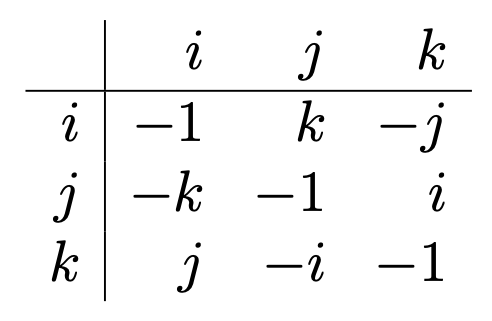
But Hamilton didn’t come at the problem by way of physics; he came at it by way of complex numbers. If having the imaginary quantity i made math richer, wouldn’t adding an independent imaginary quantity make math richer still? Hamilton sought a way to multiply numbers of the form r + ai + bj, where r, a, and b are ordinary real numbers and i and j are two independent imaginary numbers. What he realized one fateful day is that he needed a third imaginary number k, equal to i times j, to get things to work out properly. Hamilton’s quaternions were numbers of the form r + ai + bj + ck which add in the straightforward way (so that r + ai + bj + ck plus r′ + a′i + b′j +c′k equals (r+r′) + (a+a′) i + (b+b′) j + (c+c′) k) and multiply in a more complicated way, governed by the distributive law and the following table:
Working out the details of his theory, Hamilton saw that as far as multiplication was concerned, quaternions written as r + ai + bj + ck cried out to have their real and imaginary parts treated separately; that is, r + ai + bj + ck cried out to be treated as (r) + (ai + bj + ck).12 He called r the scalar part of the quaternion and ai + bj + ck the vector part.
When one separates scalars from vectors, the quaternion product of (r) + (ai + bj + ck) and (r′) + (a′i + b′j + c′k) turns out to have four parts: the scalar (r) (r′) (an ordinary product of two real numbers); the vector (r) (a′i+ b′j + c′k) = (ra′) i + (rb′) j + (rc′) k; the vector (r′)(ai + bj + ck) = (r′a) i + (r′b) j + (r′d) k; and the quantity (ai + bj + ck) (a′i + b′j + c′k), which could itself be split into two parts, namely, the scalar part
− (aa′) − (bb′) − (cc′)
and the vector part
(bc′ − cb′) i + (ca′ − ac′) j + (ab′ − ba′) k .
The first of the two is the negative of the quantity that Grassmann had called the linear product and the second is essentially the same as Grassmann’s geometric product.13
Hamilton and Grassmann were kindred spirits, multilingual polymaths with diverse interests beyond mathematics. Both came up with wildly original theories that turned out to overlap in several key places. Both initially introduced their theories in books that began with philosophical prefaces that obscured their mathematical ideas. Yet quaternions caught on and Grassmann’s theory of extensions did not. I think the main reason was that Hamilton was already famous when he came up with quaternions; people assumed that anything that the great Hamilton deemed important must be worth learning about. In contrast, Grassmann was an unknown, and it’s easier to ignore revolutionary ideas when they come from someone you’ve never heard of.14
PLUS MEN VERSUS MINUS MEN
The American scientist Josiah Willard Gibbs was initially smitten with quaternions, and in this he wasn’t alone; most of the people who later became “anti-quaternionists” were quaternionists to begin with, and they even accorded great credit to Hamilton for having invented quaternions. But they had noticed that for most scientific purposes, the quaternion product as such wasn’t very useful; only through its main constituents, the scalar product and the vector product, did it seem to play a role. Gibbs proposed that the Hamilton’s vector product of two vectors v and w be called the cross product and be denoted by v × w, and that Hamilton’s scalar product of the two vectors be called the dot product and be denoted by v · w. (Hereafter I’ll follow Gibbs and use the word “vector” instead of the word “step”.)
A close ally of Gibbs was the mathematician-physicist Oliver Heaviside, who had started as a practical electrician before he became a theoretical one, and who independently came up with the same symbols for the two kinds of products. Many years after passing through his own phase of youthful quaternionic infatuation, Heaviside wrote, “I came later to see that, so far as the vector analysis I required was concerned, the quaternion was not only not required, but was a positive evil of no inconsiderable magnitude.” Disenchanted believers often make the best apostates.
On the other hand, the mathematician Peter Guthrie Tait, the chief champion of quaternions after Hamilton’s death in 1865, was sure that quaternions were part of the architecture of the universe, and that if the dot product and cross product seemed to be strange bedfellows, that was only because physicists hadn’t constructed the right bed yet.
James Clerk Maxwell, arguably the most important physicist of that era, was a fan of quaternions. Inspired in part by the quaternionic perspective, Maxwell unified the theories of electricity and magnetism, and arrived at a startling prediction: there should be self-sustaining waves of electromagnetic oscillation in the all-permeating fluid called the æther15 that traveled at the speed of light. Maxwell became a very big deal after physicist Heinrich Hertz verified the existence of electromagnetic waves (which we now know to be the various forms of light). Maxwell’s interest in quaternions led many of his contemporaries to learn about quaternions, but many of those contemporaries, especially the physicists, became disenchanted after a time.
In the 1890s and into the early 1900s, a dozen mathematicians and physicists jousted with one another in public over the merits of quaternions. It has become common to call the anti-quaternionists “vectorialists” (which hardly seems fair since the word “vector” came from Hamilton’s work on quaternions). Just as the names of the homousian and homoiusian creeds of early Christianity differed in just a single letter, one might say that the difference between the quaternionists and their antagonists could be summarized by a minus sign. The quaternionic version of the scalar product of the triples (a, b, c) and (a′, b′, c′) was −aa′−bb′−cc′; the minus signs were an essential feature of Hamilton’s setup, since the imaginary quantities i, j, and k were square roots of −1. But physicists were finding the quantity aa′+bb′+cc′ far more useful, and had a hard time stomaching the claim that this natural-looking expression should be viewed as originating from the less useful −aa′−bb′−cc′. The mathematician and physicist Alexander MacFarlane, claiming to be above the fray rather than a part of it, nonetheless wrote that the burden of proof “lies on the minus men”.
In 1891, Gibbs remarked in the magazine Nature that, unlike quaternionic analysis, vector analysis could be extended without difficulty to higher-dimensional spaces. He saw this as a plus for vectors and a minus for quaternions. But Tait saw things differently, and demanded “What have students of physics, as such, to do with space of more than three dimensions?”
You’re probably aware that some physicists have proposed that we actually live in a space with more than three dimensions but that for various reasons those extra dimensions aren’t readily observed. Such theories are serious contenders for a Theory of Everything, so Tait’s rejoinder sounds a bit old-fashioned to modern ears. Meanwhile, vectors have proved to be useful to far more people than just physicists. In particular, computer scientists have made amazing strides in recent decades by using high-dimensional vectors. Recommendation systems that tell you what movie to watch next may be representing movies by vectors that encode salient cinematic attributes numerically and use dot-products to compute the angles between such vectors, as a way of measuring how similar they are; see the articles https://en.m.wikipedia.org/wiki/Cosine_similarity and https://tivadardanka.com/blog/how-the-dot-product-measures-similarity. More recent advances in machine learning have built on the notion of high-dimensional vectors by way of the concept of support-vector machines. And one of the most powerful approaches to machine learning is the idea of gradient descent – a deeply vectorial idea. I can’t resist mentioning that ∇, the symbol for the gradient, comes from Hamilton. So even as the role of quaternions in science has waned, the broader impact of Hamilton’s work continues to expand, and promises to continue to do so as artificial intelligence advances at its current blistering pace.
But getting back to the late 19th century: Various attempts were made to reconcile the quaternionist camp with the vectorialist camp by devising a notation that would use the best features of both. Unfortunately everyone had a different idea about what such a compromise should look like. Mathematician and physicist Alexander McAulay noted that there were nearly as many vectorial systems as there were vectorialists. He urged that the “woefully small” community of vector analysts, in the cause of advocating vectorial methods, should limit themselves to just two systems. “Let me implore them to sink the individual in the common cause.”16
Meanwhile, there were people like the mathematical physicist William Thomson, also called Lord Kelvin, who fit into neither camp – not because like MacFarlane they saw themselves as mediators but because they thought that both the quaternionists and the vectorialists had gotten caught up in a fad and lost sight of the primacy of good old reliable real numbers. After all, when one does research in the lab, what one sees on measuring devices are numbers, not vectors or quaternions. “’Vector’ is a useless survival, or offshoot from quaternions, and has never been of the slightest use to any creature,” wrote Thomson. Thomson liked to write his physics equations in triples, with one equation for Fx (the force in the x-direction), another very similar equation for Fy, and (in case one hadn’t noticed the pattern yet) a third equation for Fz. A little redundancy seemed preferable to the introduction of newfangled abstractions.17
What Thomson doesn’t seem to have appreciated is the way in which expressing proposed laws of the universe in vectorial form forces us, without any extra effort on our part, to respect the symmetries that appear to be baked into reality. Our universe seems to be rotationally symmetric as far as its fundamental laws are concerned. There is no preferred axis in physics, let alone a preferred trio of mutually perpendicular axes; if we write down a random threesome of equations, there’s little chance that the solutions to those equations will exhibit the rotational symmetry we have come to expect. On the other hand, if we write down proposed laws in vectorial form, our vectorial equations may fail to describe the universe, but they will be forced, by the very nature of vectors, to manifest rotational symmetry.
As an example of something that the vector-language of Gibbs and Heaviside doesn’t let us talk about, consider the Hadamard product operation, defined by [x, y, z] ◦ [x′, y′, z′] = [xx′, yy′, zz′]. On its surface this looks like a natural enough vectorial counterpart of the dot product of two vectors; you’d think it could be useful for physics, but it isn’t.18 The fact that vector analysis doesn’t give us a way to express this operation in terms of the operations of Gibbs and Heaviside seems at first like a liability, but it’s actually a strength. The Hadamard product doesn’t arise in physics (or Euclidean geometry), so we should be glad that our notation steers us away from it.
The abstract language of vectors – the language of addition and the two kinds of multiplication (or three, if you count the kind that stretches a vector by a scaling factor) – appears to be part of the operating system of reality; if we wish to plumb that reality, we must learn to speak and think vectorially. Vectorial concepts point us (pun intended) in the right direction.
AND HERE WE ARE
The Gibbs-Heaviside notation ultimately won out (see the Stack Exchange thread Origin of the dot and cross product) so that Maxwell’s original 20 equations governing electromagnetism got slimmed down to the four commonly written nowadays. And just as the fracas over quaternions and vectors was dying down, Maxwell’s equations gave rise to Einstein’s theory of special relativity, which in its own way sounded a death-knell for the grander ambitions of quaternionists. Hamilton thought that his three-plus-one dimensional quaternions (three dimensions for the imaginary components and one dimension for the real component) had something profound to teach us about our universe with its three dimensions of space and one dimension of time. Einstein showed that Hamilton was both right and wrong; space and time could be viewed as a unified whole, but Hamilton’s space-time was mathematically different from Einstein’s space-time, and the latter is the one that we live in. Amusingly, the battle between the plus men and minus men was echoed by a tiff that smolders to this day: should Einstein’s space-time (also called Minkowski space) be viewed as having three plus dimensions and one minus dimension or as having three minus dimensions and one plus dimension?19
An important part of the story linking Maxwell to Einstein is that Einstein and other physicists noticed that Maxwell’s equations, in addition to possessing rotational symmetry, exhibited other symmetries not explainable in pre-relativistic terms. These symmetries are called Lorentz transformations, and they were major clues that led Einstein to propose that the speed of light must be the same for all observers, even if that proposal required that the concept of speed (and with it the concepts of space and time) be updated.
In an ironic and inadvertent fashion, Einstein made another contribution to the vectorial cause in his subsequent development of general relativity. To formulate his ideas about gravity and geometry, Einstein needed something even more abstract than vectors, namely tensors. Once physicists had to come to grips with tensors, they no doubt had renewed appreciation for the comparative simplicity and concreteness of vectors. (By the way, are you wondering who invented the word “tensor”? Hamilton yet again.)
But Einstein wasn’t the first physicist to use tensors; they had already been used for decades by materials scientists to study stresses in materials like steel. Remember Leibniz’ vision of a geometry of situation that would allow one to compute the qualities of materials? Just over two centuries after he tried to interest Huygens in his vision, his vision became a reality.
As for Leibniz’s more ambitious dream of an oracle to answer humanity’s most pressing questions, it’s not clear how close we are. We used to think that digital computers (using the binary system that Leibniz championed) would make artificial intelligence possible. Nowadays we use those binary intelligences to simulate schematic brains, and devote lots of computer power to determining the weights of connections between one schematic neuron and another, using vectorial mathematics in the process. (Sometimes “vector” is just a fancy word for “list”, but the algorithms of deep learning really do take the multidimensional-space idea seriously.)
Many people these days are hopeful that that the current crop of artificial neural networks, or their successors in the not-too-distant future, will be able to assist with pressing problems in healthcare, the environment, manufacture, and education, and even help us answer basic scientific questions. But we’re still far from Leibniz’s “Let us calculate!” dream. To be sure, when we ask an AI a question, it will give us an answer, but is it the right answer? Or even a plausible one? When I gave ChatGPT the geometry problem from Endnote 4, asking it for the ratio of segments AF and FG, it produced a glib and self-assured proof that the ratio of the two lengths is −1, which isn’t a ratio of any two lengths.
So right now, we’re stuck at the “Let us chat!” stage, and it’s worth remembering that the Latin word for “chat” is confabulare, from which a different English word is derived.
Thanks to John Baez, Jeremy Cote, Evan Romer, and Glen Whitney.
This essay is a draft of chapter 9 of a book I’m writing, tentatively called “What Can Numbers Be?: The Further, Stranger Adventures of Plus and Times”. IIf you think this sounds cool and want to help me make the book better, check out http://jamespropp.org/readers.pdf. And as always, feel free to submit comments on this essay at the Mathematical Enchantments WordPress site!
ENDNOTES
#1. Leibniz wrote AB ♉︎ CD to signify that line segment AB is congruent to line segment CD. He then defined the sphere with center O and radius OP as the set of all points Q with OQ ♉︎ OP and the plane midway between points A and B as the set of all points C with AC ♉︎ BC. And so on for lines, circles, triangles, etc.
#2. Wessel is mostly remembered by mathematicians (if they remember him at all) as someone who, years before Gauss was born, figured out how to represent complex numbers using points in the plane, and how addition of complex numbers could be expressed geometrically. Less well-known is the fact that, having discovered how to add complex numbers as points in the plane via the parallelogram law, Wessel realized that there was no obstacle to adding points in three dimensions in an analogous way. Wessel applied his three-dimensional addition law to spherical trigonometry, an important tool in navigation. He presented his ideas before the Royal Academy of Denmark in 1797 and published a memoir under the auspices of that society in 1799. It was forgotten about until 1897. Mathematical historian Michael Crowe (on whose book A History of Vector Analysis I have depended heavily in the writing of this essay) describes Wessel’s memoir thus: “If it is viewed as a creation of the late eighteenth century, it can only be viewed with awe.”
#3. Here “calculus” is used in its old sense, meaning a method of calculation, and has nothing to do with the differential and integral calculus of Leibniz and Newton. “Barycenter” means “center of gravity” or “center of mass”.
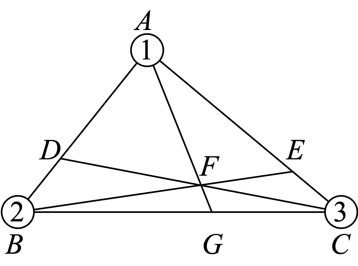
#4. For instance, consider the following problem: “Given a triangle ABC, point D is drawn on side AB so that AD is twice as long as DB and point E is drawn on side AC so that AE is three times as long as EC. Let point F be the intersection of lines BE and CD, and let point G be the intersection of lines AF and BC. What is the ratio of the length of AF to the length of FG?” To solve this problem with mass point geometry, no genius is required, and not even a lot of writing; a mass-point adept can draw the picture shown below (signifying putting 1 unit of mass at A, 2 units of mass at B, and 3 units of mass at C), read off the answer to the problem as (2 + 3) : 1 (a ratio of five-to-one), and move off to the next problem while non-adepts are still scratching their heads. To become an adept, check out the article by Sitomer and Conrad listed in the References.
#5. For a discussion of what negative weights might have meant to Möbius, see the History of Science and Mathematics Stack Exchange thread Negative coefficients in the barycentric calculus.
#6. The 19th century bestseller Common Sense of the Exact Sciences started out as a solo project in which Clifford aimed, among other things, to give a simplified presentation of Grassmann’s ideas, as Clifford had expounded them in a more technical 1885 book. Clifford died in the course of the project and it was completed by Pearson, who among other things wrote the chapter on vectors. Pearson’s “rho” (ρ), a measure of statistical correlation he popularized ten years later, can be interpreted as the cosine of an angle between two vectors in a high-dimensional space; the interested reader can learn about this connection in chapter 15 of Jordan Ellenberg’s 21st century bestseller How Not To Be Wrong.
#7. Some readers may find it helpful to recall a formula often taught in high schools for the area of parallelogram whose vertices are given in Cartesian coordinates. Specifically, a parallelogram with vertices (0, 0), (a, b), (c, d), and (a+c, b+d) has area ad−bc, provided the closed path from (0, 0) to (a, b) to (a+c, b+d) to (c, d) to (0, 0) goes counterclockwise; if instead the path goes clockwise, then ad−bc is the negative of the area. This is simplest to see in the case (a, b) = (1, 0) and (c, d) = (0, 1) (which gives ad−bc = +1) and the case (a, b) = (0, 1) and (c, d) = (1, 0) (which gives ad−bc = −1).
#8. Look up “bivector” if you want to know the right way to think about the geometric product. And if you really want to be technical, you should know that the geometric product of two steps in the plane isn’t a signed number either, but a vector in a one-dimensional space.
#9. Consider a right triangle with legs AB and AC, represented by the steps s and t as shown.
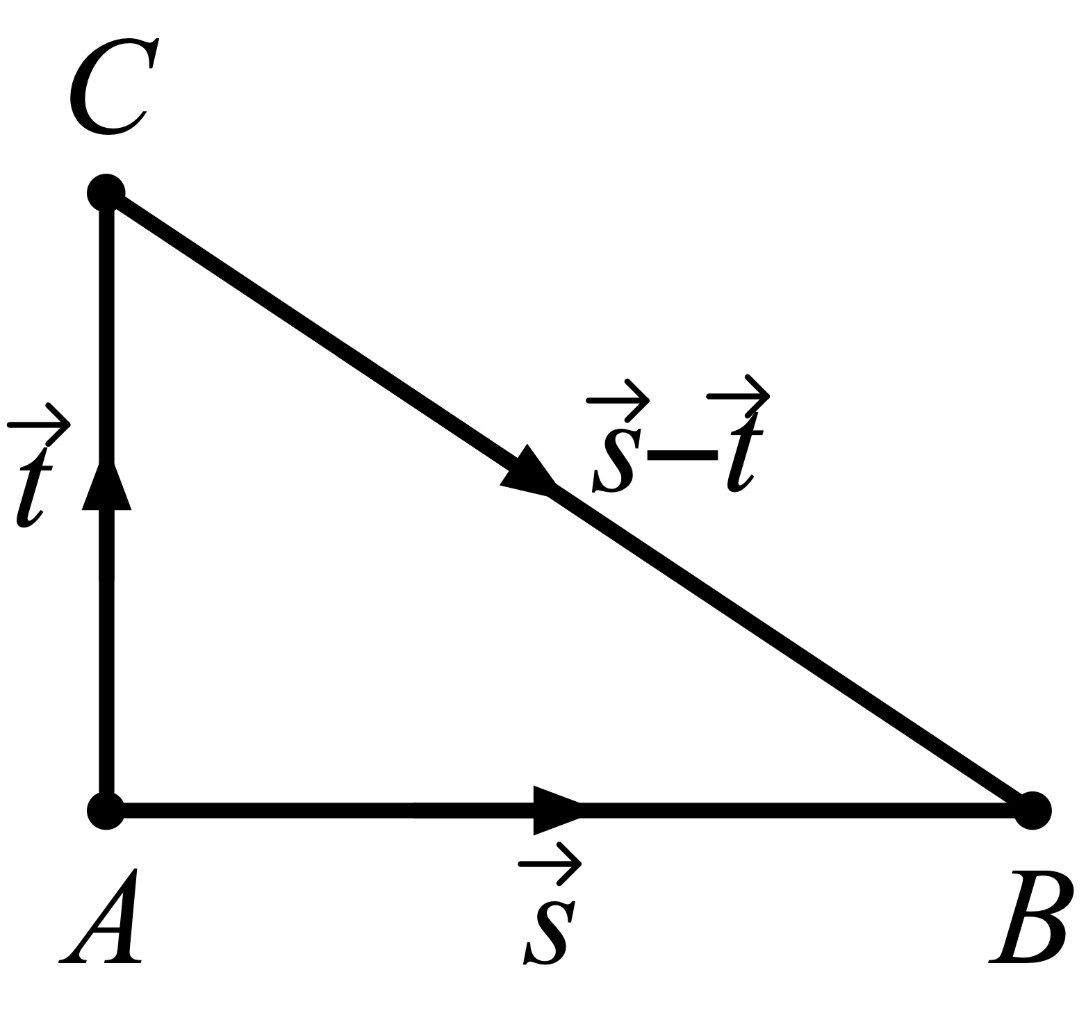
Then the hypotenuse corresponds to the step s − t, so the squared length of the hypotenuse is (s − t) · (s − t). Applying the distributive law a couple of times, we write this as s · s − s · t − t · s + t · t. But the middle two terms equal 0 (because s · t = 0 when s and t are orthogonal), so we’re left with s · s plus t · t. The first of these is the squared length of s and the second is the squared length of t, so the squared length of the hypotenuse of a right triangle equals the sum of the squared lengths of the legs.
#10. Consider parallelogram ABCD as shown, with s = A→B = D→C and t = A→D = B→C.
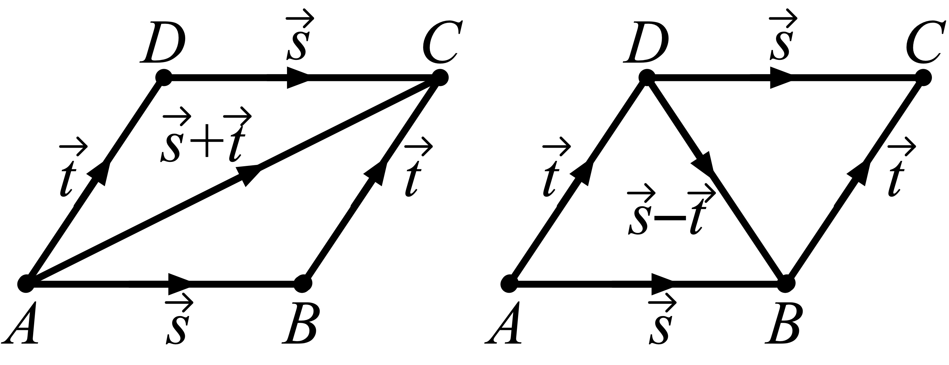
One of the diagonals is given by s + t while the other is given by s − t, so the sum of the squared lengths of the diagonals is (s + t) · (s + t) + (s − t) · (s − t). If we expand this using the distributive law, we get the eight terms
s · s + s · t + t · s + t · t + s · s − s · t − t · s + t · t ,
but four of those terms cancel, leaving just
s · s + t · t + s · s + t · t
which is indeed the sum of the squared lengths of the four sides.
#11. One can decree points in n-dimensional space to be n-tuples of real numbers, define distance between points and angles between lines using the linear product, and define areas and volumes using the geometric product. Even if we can’t visualize objects in these spaces, we can still compute their properties using Grassmann’s formulas.
#12. Later Hamilton adopted a more geometrical view of quaternions and came to wish he’d presented that symmetrical picture first without bringing i, j, and k into the story.
#13. More specifically, the magnitude of (bc′ − cb′) i + (ca′ − ac′) j + (ab′ − ba′) k is the same as the magnitude of the geometric product of [a, b, c] and [a′, b′, c′], and the direction of (bc′ − cb′) i + (ca′ − ac′) j + (ab′ − ba′) k is perpendicular to the plane spanned by [a, b, c] and [a′, b′, c′].
#14. Fortunately Grassmann did receive recognition in his own lifetime, though not until his final years.
#15. Maxwell, like most of his contemporaries, was wrong about the æther, but he was right about the waves.
#16. There was a commission in 1903 set up specifically to choose the best symbolism for vector analysis; the only result of the activity of the commission was that three new notations came into being.
#17. For more on Thomson’s quarrel with vectors, see the Straight Dope post Why did Lord Kelvin think vectors were useless?
#18. To see why the Hadamard product is geometrically unnatural, compare the vectors v = [1,1,1] and w = [sqrt(3),0,0]. There’s a rotation that brings v to w (since v and w are both vectors of magnitude sqrt(3)) so the two vectors should have the same properties; but v ◦ v = v whereas w ◦ w ≠ w. Thus the Hadamard product, unlike the dot and cross products, doesn’t exhibit rotational symmetry. Putting it differently: if we lived in a universe where the Hadamard product was an essential ingredient in the mathematical expression of physical laws, there would have to be a preferred coordinate frame. No such frame exists in our universe.
#19. My remark about plus dimensions and minus dimensions makes more sense if you know about the metric signature of spacetime.
REFERENCES
William Clifford and Karl Pearson, The Common Sense of the Exact Sciences, 1885
Michael J. Crowe, A History of Vector Analysis, 1967
David Miller, The Parallelogram Rule from Pseudo-Aristotle to Newton, Archive for History of Exact Sciences, vol. 71, no. 2 (March 2017), pp. 157– 191
Harry Sitomer and Steven Conrad, Mass Points, Eureka (aka Crux Mathematicorum), vol. 2, no. 4 (April 1976), pp. 55–62
