Bertrand’s Ballot Problem

Early leads don’t always lead to much. Remember Republican presidential candidate Rudy Giuliani? Back in 2008, the outspoken New Yorker polled so well that some pundits predicted he’d win the nomination, but his lead fizzled out before the convention. The same thing has happened with many other would-be presidents from both sides of the aisle over the past couple of decades. So you might be inclined to discount a candidate’s early lead in polls. In fact, this reasonable inclination was part of why FiveThirtyEight analyst Harry Enten didn’t see Donald Trump’s nomination coming; Enten figured that Trump would wind up being just another Giuliani. Oops.

So, how closely do we expect early polling in an election process to correspond with the final outcome? A classic problem in probability theory strips this real-world question down to manageable size.

In the late 19th century, French mathematician Joseph Bertrand imagined an idealized election process in which there are just two candidates, A and B. Suppose p of the voters picked A and q of the voters picked B, with p > q. Suppose also that, after the voting ends, the ballots (which have been scrambled to remove all vestiges of order) are counted one at a time. Bertrand asked: What’s the chance that candidate A will be strictly ahead of candidate B throughout the count?

Let me clarify the question with the simple example p = 2, q = 1. There are three equally-likely possible orders in which the three votes (2 for A and 1 for B) could be tallied:

AAB: A pulls into the lead after the first ballot and stays in the lead thereafter: yay!
ABA:  A starts with a lead but loses it before regaining it: not so yay
BAA: A isn’t in the lead until the last ballot is read: even less yay

Only one the three scenarios has candidate A staying in the lead throughout the count, so the chance that A is in the lead throughout, given that p = 2 and q = 1, is exactly 1/3.

Note that I could have asked a slightly different question, in which “ABA” would count as a “yay” because candidate A doesn’t actually ever fall behind; after two ballots have been counted, it’s a tied race. But that’s not the question Bertand was asking.

If you’re awfully anxious to know the answer (“Bertrand’s Ballot theorem“), you can peek at the end of this essay. But I want to focus not on the answer, but on the kind of reasoning that’s involved in proving the formula. It’s a great application of combinatorics to probability, with a dash of dynamical systems flavoring thrown in.

MAXIMIZING DRAMA

To make things as dramatic as possible, and to make the scenario easier to think about, let’s focus on the case where A’s victory is as narrow as possible. Suppose n+1 people voted for candidate A but only n people voted for candidate B. Let’s start with a qualitative question: Which do you think is more likely — that (1) throughout the tallying, A will have a majority of the already-tallied votes? — or, at the other extreme, that (2) throughout the tallying, A will never have a majority of the already-tallied votes, until the fateful moment when the final ballot is tallied?

I think most people intuitively feel that the first probability should be larger, even if only slightly. After all, the electorate is tilted slightly in favor of A, isn’t it? But remember that winning exactly half of the already-tallied votes doesn’t count as winning a majority of the already-tallied votes; if, at some point in the counting, equal numbers of ballots for A and for B have been counted, neither candidate has a majority of the already-counted votes. Do you still think probability (1) is larger? Or does the stringency of the meaning of “majority” make you think that probability (2) is larger?

If you think this question is too close to call — if your intuitive sense is that those two probabilities are close to each other — you’ve got good intuition. Because, in fact, the two probabilities are equal.

Before I explain why they’re equal, no matter how big n is, let’s check that what I claimed is true for small values of n. I’ll list all the different orders in which the 2n+1 ballots can be read, and I’ll mark a specific ballot-order with a yellow smiley face if the winning candidate maintains a majority throughout the tallying, with a red frowny face if the winning candidate doesn’t ever manage to pull ahead until the end, and with “…” if the outcome falls between those two extremes.

First, let’s look at the case n = 1 again, this time with faces:

AAB:
ABA:  …
BAA: 

There are three equally likely outcomes: one “smiley”, one “frowny”, and one neither. So the probability that the winning candidate maintains a majority throughout the tallying (“P” for short) is 1/3, as is the probability that the winning candidate doesn’t pull ahead until the end (“P” for short).

Next, let’s look at the case n = 2 (with 3 votes for A and 2 votes for B):

AAABB:
AABAB:
AABBA: …
ABAAB: …
ABABA: …
ABBAA: …
BAAAB: …
BAABA: …
BABAA: 
BBAAA: 

Since there are 10 equally likely orders in which the ballots can be read aloud, 2 of the “smiley” kind and 2 of the “frowny” kind, we get P = 2/10 and P = 2/10 as well.

So now you’ve seen that P = P for n = 1 and for n = 2. Try to prove that P = P for all values of n, or else keep reading!

A SYMMETRY ARGUMENT

The trick is to notice that, just as “every frown is a smile turned upside down”, every frowny ballot-order is just a smiley ballot-order turned backwards. Look back at the table for n = 2: if you take the two frowny ballot-orders from the bottom of the table (BBAAA and BABAA) and turn them backwards, you get AAABB and AABAB: the two smiley ballot-orders from the top of the table! That’s no accident: the same thing happens for n = 3, n = 4, etc. We’ll prove that the number of rows that get marked with a smiley must equal the number of rows that get marked with a frowny. And that means that P must equal P , even if we don’t (yet) know the value of either of these numbers.

It’ll help to switch to a pictorial way of thinking about the tallying process. We’ll represent each ballot-order by a graph that shows the evolution over time of candidate A’s lead, defined as the number of already-counted votes for A minus the number of already-counted votes for B; this quantity can be positive, negative, or zero. Consider for instance the ballot-order ABBABAA; starting from when 0 votes have been counted, and ending when all 7 votes have been counted, we see candidate A’s lead take the successive values 0,1,0,−1,0,−1,0,1, giving the graph shown in Figure 1.

Figure 1

As we view the zigzag-shaped graph from left to right, each upward stroke corresponds to a vote for A while each downward stroke corresponds to a vote for B. I’ve drawn a dashed line joining the leftmost and rightmost points on the graph, for reasons I’ll explain later. The marked points along the graph are lattice points: points (x,y) where the horizontal coordinate x and the vertical coordinate y are both integers.

A smiley ballot order is one whose graph stays above the dashed line except at the two ends. A frowny ballot order is one whose graph stays on or below the dashed line except at the two ends. (See Endnote #1 to understand why the dashed line plays this crucial role.) The ballot order ABBABAA, depicted in Figure 1, is neither smiley nor frowny, since its graph visits both sides of the dashed line.

Here’s a picture showing the graph for the ballot order AAABABBAB:

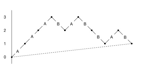
Figure 2.

It’s a smiley ballot order: the graph stays above dashed line.

If we reverse the order of the ballots, we get the ballot order BABBABAAA, whose graph is shown in Figure 3.

Figure 3.

This is just the previous picture, turned around! That is, if you print Figure 2 on a piece of paper and give it a half-turn, then (ignoring the coordinate axes) you’ll see Figure 3. Stop a minute to convince yourself that this is no accident.

If you apply a half-turn to a picture of a graph that stays below a dashed line, you get a picture of a graph that stays above a dashed line, and vice versa. So, reversing a smiley ballot-order gives a frowny ballot order, and vice versa. This gives us a one-to-one correspondence between the smiley rows of the table and the frowny rows of the table, so there must be exactly as many smiley ballot-orders as frowny ballot-orders.

DISCRETE DYNAMICS

We’ve shown that P = P for all n, but can we find a formula for this probability?

We already saw that when n is 1, P is 1/3, and that when n is 2, P is 2/10. I’ll save you some time and tell you that when n is 3, P is 5/35; that when n is 4, P is 14/126; and that when n is 5, P is 42/462. See a pattern?

If you wrote those fractions in reduced form as 1/3, 1/5, 1/7, 1/9, and 1/11, you no doubt guessed that P is 1/(2n+1). But why should this be true?

To see what’s going on, we’ll play a different game with ballot-orders: given a string of A’s and B’s, we’ll take the first symbol in the string and move it to the end. For instance, if we take the ballot-order AAABB and apply the move-the-first-letter-to-the-end operation, we get the ballot-order AABBA. If we do it again, we get ABBAA. Doing it again gives BBAAA. Doing it again gives BAAAB. And doing it for a fifth time brings us back to AAABB. This accounts for five of the ten ballot-orders that can occur when n = 2. What about the other five? Pick one of them, say AABAB. If we apply the move-the-first-letter-to-the-end operation over and over, we successively get ABABA, BABAA, ABAAB, BAABA, and then AABAB again. All ten of the ballot-orders have been included in the dance, diagrammed in Figure 4.

Figure 4.

This dance is an example of a discrete dynamical system. It’s discrete in two ways: the flow of time has been discretized, and the set of configurations that we’re allowing is finite. (Compare with the idealized oscillation of a mass attached to a spring in one dimension: the state of the system is determined by the position and momentum of the mass, so we imagine the state of the system at any instant as being a point in a two-dimensional phase space, and the time-evolution of the physical system is represented by a trajectory in phase space. For our mass-on-a-spring system, the state space is infinite and time is continuous.) Also notice that the “time” we’re talking about in our discrete dynamical system, associated with the arrows in Figure 4, is not the kind of time that elapses as the ballots are read aloud in succession (associated with the horizontal axes in Figures 1 through 3); the arrows represent a more abstract kind of time that is not native to the problem but which the mathematician is introducing as a form of conceptual leverage. This fictional time has the property that after five ticks of the clock, the system is back exactly to where it started.

A general feature of dynamical systems is that they divide the phase space into orbits; as the system evolves, the point in phase space (also called state space) that represents the state of the system travels along an orbit. In our case, we have a ten-element phase space, and the dynamics divide it into two orbits, one consisting of the states AAABB, AABBA, ABBAA, BBAAA, and BAAAB and the other consisting of the states AABAB, ABABA, BABAA, ABAAB, and BAABA.

More generally, if we look at all the ways to order n+1 ballots for A and n ballots for B (represented as strings of n+1 A’s and n B’s), and our dynamics are given by the move-the-first-letter-to-the-end operation, then our phase space gets divided up into orbits, all of which have size exactly 2n+1. (It’s pretty clear that no orbit can have size bigger than 2n+1: no matter what state you start in, if you apply the operation 2n+1 times, you get back to where you started. But how do we know that you don’t get back to where you started sooner than that? See Endnote #2.)

What’s the payoff of looking at things this way? This simple fact (whose proof is coming up): Each orbit contains exactly one smiley ballot-order. (Each orbit also contains exactly one frowny ballot-order.) Check it out:

AAABB:
AABBA: …
ABBAA: …
BBAAA:
BAAAB: …

AABAB:
ABABA: …
BABAA:
ABAAB: …
BAABA: …

This is a special case of the cycle lemma (sometimes called Raney’s lemma); see the article by Dershowitz and Zaks listed in the references.

A PICTORIAL PROOF

To see why each orbit contains exactly one smiley ballot order (and exactly one frowny ballot order), let’s reexamine the ballot order ABBABAA that we saw in Figure 1. If what I’ve told you is true, the orbit of ABBABAA consists of seven ballot orders, one of which is smiley and one of which is frowny. Let’s find them pictorially! To do this, take copies of the graph shown in Figure 1 (including the dashed line) and repeat it over and over, so that it extends out to infinity in both directions:

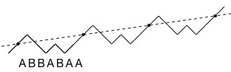
Figure 5.

As before, A means upward and B means downward as we scan from left to right. I’ve broken up the infinite path into finite paths by using dots as dividers, to remind us of what Figure 1 looked like. Figure 5 now represents all members of the orbit, depending on where you choose to start. Now imagine taking that dashed line and sliding it downward (without changing its slope) until it just barely grazes the bottom of the zigzag path:

Figure 6.

I’ve marked the points of contact between the shifted line and the zigzag path with dots. If you read off the letters on the path-segments that join each dot to the next, you get AAABBAB: the smiley member of that orbit.

Now imagine taking that dashed line and sliding it upward until it just barely grazes the top of the zigzag path:

Figure 7.

If you read off the letters on the path-segments that join each grazing point to the next, you get BBABAAA: the frowny member of that orbit.

This works for any n: each orbit has size 2n+1 and contains exactly 1 smiley ballot-order and exactly 1 frowny ballot-order. That’s why the proportion of smiley ballot-orders overall is exactly 1 divided by 2n+1. (Here’s an analogy: If a town in China consists of nothing but 2-parents-plus-1-child families, then 1/3 of the residents of the town must be children. In this analogy, the division of the residents into families of size 3, with one child per family, is analogous to the way the dynamics divide the phase-space into orbits of size 2n+1, with one smiley member of each orbit.)

CHUNG AND FELLER

Being smiley and being frowny are just two endpoints of a spectrum. Define the smileyness of a ballot-order as the number of times in the ballot-tallying process when candidate A is in the lead. This number could be as big as 2n+1 (if the ballot order is smiley) or as small as 1 (if the ballot is frowny), or it could be anything in between. We’ve seen that if you tally ballots in a random order, the probability that the smileyness equals 1 is 1/(2n+1), and the probability that the smileyness equals 2n+1 is also 1/(2n+1). What can be said about the probability that the smileyness is k, where k is some value between 1 and 2n+1?

Twentieth-century mathematicians Chung and Feller showed that, regardless of the value of k, the probability that the smileyness of a ballot will be equal to k is always the same number: 1/(2n+1). One nice way to prove this is to show that in each orbit of our dynamical system, each of the numbers 1,2,…,2n+1 occurs exactly once. Here’s a verification for the case n=2.

AAABB: 5
AABBA: 4
ABBAA: 2
BBAAA: 1
BAAAB: 3

AABAB: 5
ABABA: 3
BABAA: 1
ABAAB: 4
BAABA: 2

Here I’ve bolded the letters that correspond to ballots with the property that, after the ballot is read aloud, candidate A is in the lead. The smileyness of a ballot-sequence is the number of bolded letters. The example bears out Chung and Feller’s theorem. You may want to try to prove the theorem on your own before you peek at Endnote #3.

A CLASSIC PUZZLE

I want to share with you a classic puzzle that hooks nicely onto the proof I just showed you. It’s usually stated in terms of a jeep, but I’ll use a motorcycle instead. There’s a long circular track in a desert that needs to be patrolled. A scout and a motorcycle are to be helicoptered to a spot along the track, and the scout must make a complete clockwise circuit of the track on the motorcycle, which has a 1-gallon tank. The helicopter pilot tells the scout, “I’ve got good news and bad news.” “What’s the bad news?” “The tank on this motorcycle is empty.” “Oh yeah? And what’s the good news?” “The good news is that there are cans of gasoline placed along the track, and together the cans contain 1 gallon of gasoline, which is just enough gasoline to get you and this motorcycle around the track one time. Here’s a map that shows where the cans are and how much gasoline each one contains. Where do you want me to drop you?”

If you’re the scout, you’d better get dropped off where one of the gasoline cans is; the question is, which gasoline can? Should it be the one containing the most gas? Not necessarily, if it’s too far away from other gas cans. Should it be the one that has the shortest distance to the next can? Not if the first can has too little gas to get the scout to the second can! Once you start pondering the problem, it’s natural to switch from pondering to worrying: How can we be sure that there is a solution? Is it possible that whoever set up the cans diabolically made it impossible for the scout to make the trip, no matter where the helicopter pilot drops her off?

Your mission: Either find such a diabolical set-up for the cans, OR show that the scout always has some way of carrying out the mission. See Endnote #4 for a solution.

BACK TO BERTRAND

Bertrand proved that if you have p people voting for A and q people voting for B, with p > q, the probability that A will always be in the lead is (p−q)/(p+q). For instance, if you have p = 7000 people voting for A and q = 3000 people voting for B, Bertrand’s formula gives P = 40%. For many effects of chance, scaling up the numbers reduces the effects of randomnesss, but this isn’t one of them. Scale the preceding scenario up by a factor of 1000 and we’re still looking at P = 40%: if candidate A gets 7,000,000 votes and candidate B gets 3,000,000 votes, there’s a 60% chance that the lead will change at least once throughout the vote-counting process.

That 60% figure seems impressive until you consider that 30% of the time, the very first vote that gets counted is a vote for B, which guarantees that a change in the lead will occur later. In fact, there’s a 59% chance that, at some point in the counting of the first ten votes, candidate B will be doing at least as well as candidate A. If instead of asking “What’s the chance that B will be doing at least as well as A at some point in the tallying process?”, we ask “What’s the chance that B will be doing at least as well as A at some point after the first ten ballots have been tallied?”, then that 60% figure drops much lower. And after one hundred ballots have been tallied, it’s overwhelmingly likely that candidate A will have the lead and never lose it thereafter. So for statistically savvy election-watchers who know that reliability increases with sample-size, and who would never think to extrapolate an election outcome based on knowing a meager fraction of the votes, Bertrand’s formula is a bit moot.

There’s another way in which Bertrand’s formula fails to help us understand Donald Trump’s candidacy: the formula assumes that the casting of all the ballots precedes a big, gradual reveal of how the public voted. But when party-voters pick delegates to represent them at a convention, it’s done state by state, and the whole nation gets to find out the outcome of last Tuesday’s primaries before next Tuesday’s primaries. This information can influence people’s decisions in all kinds of ways, and Bertrand’s model completely ignores these influences.

Yet another disconnect between Bertrand’s formula and the real world is that Bertrand’s problem isn’t about what really matters, namely, predicting the outcome of an election based on information that dribbles in over time. Bertand’s formula is about the opposite! That is, it’s about predicting the information-dribble based on the eventual outcome. Remember that Bertrand takes the numbers p and q as givens. In a real election, p and q aren’t givens; they’re the last thing one learns. Estimating p and q from early polling is the kind of thing Nate Silver and Harry Enten and other applied statisticians do, but Bertrand was proving a theorem in probability theory. In probability theory, we ask “Given that hypothesis H is true, what sort of data D should we expect to see?” In statistics, we ask “Given that we’ve seen data D, should we believe hypothesis H?” The problems are related, but they are not the same.

So, why have I written this essay? Partly because its theme seemed topical. But also because I love the way you can use pictures to show that P = 1/(2n+1). I first learned a version of this proof when I was in high school, from Yaglom and Yaglom’s book (see the references). The first time one sees arguments like this, one may think “How wonderfully clever!”, or “How depressingly clever; I could never come up with something like that.” But after one’s initial emotion reaction to seeing the “magic trick” has receded, the right thing to do is ask oneself “How can I recognize other situations in which this trick, or something like it, will work?” So I’ll wrap up this essay by asking: For what values of p and q does the trick work? And, when it doesn’t work, how can you prove that Bertrand’s formula still holds?

Thanks to Félix Balazard, Sandi Gubin, Scott Kim, Andy Latto, Fred Lunnon, Henri Picciotto, Ted Propp, James Tanton, and Glen Whitney. Also thanks to the kind folks at Omni Group Tech Support who helped me take my first steps in using OmniGraffle.

Next month (Sept. 17): Going Negative.

ENDNOTES

#1: When is a string of n+1 A’s and n B’s smiley? When its graph (which starts at (0,0) and ends at (2n+1,1)) stays above the line y=0 except at (0,0). But since the right triangle with vertices (0,0), (2n+1,0), and (2n+1,1) doesn’t contain any lattice points in its interior between the line y = 0 and the line y = x/(2n+1), a zigzag lattice path from (0,0) to (2n+1,1) stays above the horizontal line y = 0 (except at the left endpoint) if and only if that path stays above the dashed line y = x/(2n+1) (except at the left and right endpoints). Get out a piece of graph paper and you’ll see what I mean.

Likewise, when is a string of n+1 A’s and n B’s frowny? When its graph stays below the line y=1 except at (2n+1,1). But since the right triangle with vertices (0,0), (0,1), and (2n+1,1) doesn’t contain any lattice points in its interior between the lines y = 1 and y = x/(2n+1), a zigzag lattice path from (0,0) to (2n+1,1) stays below the horizontal line y = 1 (except at the right endpoint) if and only if that path stays below the dashed line y=x/(2n+1) (except at the left and right endpoints).

#2: Say we have a string of n+1 A’s and n B’s, and we move the first k symbols to the end, leaving them in the same order, where 0 < k < 2n+1. (That’s equivalent to performing the move-the-first-symbol-to-the-end operation k times.) How can we be sure that the new string is different from the one we started with? (We need to know this if we want to know that each orbit is really of size 2n+1.)

There are ways to prove this directly, but I like to derive it as a consequence of the analysis that proves the Chung-Feller theorem! Details appear below.

#3: Start with a grazing line like the dashed line shown in Figure 7. We’ve already seen that if you read the letters on the zigs and zags between two successive points of contact between the grazing line and the zigzag path, you get a ballot-order of smileyness 1 (we called it “frowny” when we showed this). Now slide this dashed line down until it goes through two new vertices of the zigzag path. If you read the letters on the zigs and zags between two successive points of contact between the relocated dashed line and the zigzag path, you get a ballot-order of smileyness 2. Keep on doing this, and you’ll successively obtain a ballot-order of smileyness 3, smileyness 4, etc.

To see that the smileyness always goes up by 1, we have to show that as we lower the dashed line, we never pick up more than 1 lattice point within any given stretch of width 2n+1. Putting it differently, a displaced dashed line parallel to the original dashed line can’t go through more than one lattice point between x = 0 and x = 2n+1 in the picture. Why can’t it go through a third lattice point? Because the slope is so close to zero. More specifically, consider the points (0,r) and (2n+1,s) lying on the dashed line (where r and s need not be integers). Because the slope of the line is 1/(2n+1), we have s = r+1. For any intervening point (x,t) on the dashed line, we have 0 < x < 2n+1, and accordingly r < t < r+1. So there’s at most one possible integer value for t that works, and hence at most one lattice point (x,t) with 0 < x < 2n+1 that lies on the dashed line.

Now you can see my covert reason for putting those divider-dots into Figure 5. You should imagine that Figure 6 morphs into Figure 7, passing through Figure 5 on the way. Each time the slowly falling dashed line passes through lattice points, a little smileyness-counter goes up by 1. Or, if your visual imagination is feeling tired today, check out Henri Picciotto’s nifty animation.

#4: The scout should draw a graph like the one shown in Figure 8, which shows the contents of the gas tank of a motorcycle that’s like the one she’s going to use, except that it has a 2-gallon tank that starts out with 1 gallon of gas in it. The scout has chosen to place the imaginary motorcycle at a place where there isn’t a can of gasoline, so as she starts to drive, her “gasoline function” immediately starts decreasing at a steady linear rate. Then the gasoline function jumps up discontinuously where the imaginary motorcycle comes to a gas can. The graph shows steady linear decrease punctuated by discontinuous jumps. The right endpoint of the graph is at the same height as the left endpoint, corresponding to the fact that the cans contain just enough gasoline to get a motorcycle around the track. The scout should identify the lowest point on this graph; the corresponding can of gasoline marks the spot where she should have the helicopter drop her and her actual, 1-gallon-capacity motorcycle.

Figure 8.

#5: If we treat all ballots for A as indistinguishable from one another, and ditto all ballots for B, the total number of different ballot orders (or equivalently, the total number of strings we can form out of n+1 A’s and n B’s) is the binomial coefficient (2n+1)!/(n!(n+1)!). We’ve seen that this set of strings can be divided into orbits of size 2n+1 (as shown in Figure 4 for the case n = 2), which tells us that the number of orbits is (2n+1)!/(n!(n+1)!) divided by 2n+1, or (2n)!/(n!(n+1)!). This number is called the nth Catalan number. It’s also equal to the number of smiley ballot sequences, since each orbit contains exactly one smiley ballot sequence. The Catalan sequence begins 1, 2, 5, 14, 42, … and it arises in mathematics in deeper and more diverse ways than even the famous Fibonacci sequence 1, 2, 3, 5, 8, 13, … Many people first learned about Catalan numbers from Scientific American, whose June 1976 issue contained Martin Gardner’s essay “Catalan Numbers”. (You can find this piece as Chapter 20 in Gardner’s book “Time Travel and Other Mathematical Bewilderments”.) See Richard Stanley’s book for much, much more about the Catalan numbers, or for a taste, the entry on Catalan numbers in the Online Encyclopedia of Integer Sequences.

#6: The proof works whenever p and q are relatively prime positive integers satisfying p > q; the set of strings you can form with p A’s and q B’s divides up into orbits of size p+q, and each orbit contains exactly one smiley string. However, this argument fails when p and q have a common factor larger than 1. For instance, with p = 4 and q = 2, the string AABAAB has an orbit of size 3; the state space consists of this orbit of size 3 and two orbits of size 6. (Relatedly, observe that when you have a ballot-sequence graph that has p up-steps and q down-steps with p, q not relatively prime, and you draw a dashed line from the start-point (0,0) to the end-point (p+q,p−q), the dashed line and the zigzag graph can have more than just their endpoints in common; they can pass through some of the same lattice points in between.) However, when p = 4 and q = 2 it’s still true that (p−q)/(p+q) of the elements of each orbit are smiley; it’s just that sometimes it’s 1-out-of-3 and sometimes it’s 2-out-of-6. A simple way to patch the proof is to think of a string like AABAAB as being two repetitions of the string AAB, so that it falls under the analysis given in the p = 2, q = 1 case (and likewise more generally). See the article by Renault.

#7: “What about Boltzmann?” (The original title of this essay, as advertised back in July, was “Ballots and Boltzmann”.) On the advice of one of my trusted pre-readers, I slimmed down this essay and removed the discussion of physical and mathematical notions of ergodicity and their relevance to Chung-Feller. Once I’ve discussed more examples of discrete dynamical systems, such as Bulgarian Solitaire, I’ll return to this topic.

REFERENCES

K.-L. Chung and W. Feller, On Fluctuations in Coin-Tossing, Proceedings of the National Academy of Sciences of the U.S.A. (1949), vol. 35, pages 605-608.

N. Dershowitz and S. Zaks, The Cycle Lemma and Some Applications, European Journal of Combinatorics (1990), vol. 11, pages 35-40.

H. Enten, What Harry Got Wrong in 2015. (See also N. Silver, How I Acted Like a Pundit and Screwed Up on Donald Trump.)

F. Mosteller, Fifty Challenging Problems in Probability With Solutions (see problem 22).

M. Renault, Four Proofs of the Ballot Theorem, Mathematics Magazine (2007), vol. 80, pages 345-352.

R. Stanley, Catalan Numbers, 2015.

A.M. Yaglom and I.M. Yaglom, Challenging Mathematical Problems with Elementary Solutions (2 volumes).